T-Distributed Stochastic Neighbor Embedding (t-SNE)

Introduction

T-Distributed Stochastic Neighbor Embedding (t-SNE) is a powerful technique for dimensionality reduction that has taken the machine learning and data visualization communities by storm. In an era of big data and high-dimensional datasets, t-SNE provides an easy approach for reducing complex data to a lower-dimensional space, enabling visualization and comprehension of the data’s underlying structure. In numerous applications, including image classification, text analysis, gene expression, and many others, t-SNE has proven to be particularly effective at revealing patterns and correlations. This potent technique has not only revolutionized the way data is represented, but it has also led the way for new insights and discoveries in a variety of sectors. In this article, we will explore the mathematics behind t-SNE, explain how it operates, and demonstrate its visualization capabilities for high-dimensional data.

t-SNE

t-SNE (t-Distributed Stochastic Neighbor Embedding) is an effective and widely-applied method for displaying high-dimensional data. It is an unsupervised machine learning technique that reduces the dimensionality of huge datasets and identifies patterns, relationships, and clusters in multidimensional and complicated data. In 2008, Laurens van der Maaten and Geoffrey Hinton introduced this approach.

How does it work?

t-SNE transforms high-dimensional data into a two-dimensional scatter plot or other low-dimensional representation. This low-dimensional representation is designed to preserve as much as possible the distance between points in the high-dimensional space in the low-dimensional space. This facilitates the visualization of the relationships between points in the high-dimensional space and reveals the data’s underlying structure.

The t-SNE algorithm defines a probability distribution across the high-dimensional data points such that the similarity between points is proportional to the likelihood that they are neighbors. It works by preserving the local and global structure of the data by mapping it to a low-dimensional representation that is optimized using the Kullback-Leibler divergence. This is accomplished by computing the conditional probability distribution across each point’s neighbors. The t-SNE then maps these probabilities to a two-dimensional scatter plot, where the distances between points correspond to the similarities in the high-dimensional space.

Math under the hood of t-SNE

The mathematics underlying t-SNE can be interpreted as follows:

1. KL Divergence: The initial step is to compute the Kullback-Leibler (KL) divergence between the high-dimensional and low-dimensional probability distributions. KL divergence is a measurement of the difference between two probability distributions. In t-SNE, the probability distributions of high-dimensional data points are compared to those of low-dimensional data points.
2. High-Dimensional Similarity: The following step is to determine the high-dimensional similarity between the data points. This is accomplished by calculating the pairwise distances between data points in the high-dimensional space.
3. Low-Dimensional Similarity: The following step is to determine the low-dimensional similarity between the data points. This is accomplished by converting the high-dimensional similarity to the low-dimensional similarity. The altered low-dimensional similarity will subsequently be utilized to construct the gradient descent update for the t-SNE optimization procedure.
4. Gradient Descent Optimization: Finally, gradient descent optimization is used to update the low-dimensional representation of the data points. This entails computing the gradient of the KL divergence with regard to the low-dimensional representation of the data points and thereafter updating the representation until convergence.

t-SNE involves minimizing the KL Divergence as:

t-SNE Objective

The objective function of t-SNE can be represented as below:

t-SNE Cost Function

where p_ij and q_ij are the probabilities that data points i and j are neighbors in the original high dimensional space and the low dimensional space, respectively. The sum over j is taken over all data points that are not equal to i.

The probability p_ij can be expressed as:

High Dimensional Spatial Probability

where x_i and x_j are the data points in the high dimensional space, and sigma_i is a parameter that can be tuned to control the variance of the Gaussian distribution used to compute the probabilities.

The probability q_ij can be expressed as:

Low Dimensional Spatial Probability

where y_i and y_j are the data points in the low dimensional space.

By minimizing the t-SNE objective, we can obtain a low dimensional representation that preserves the structure of the data. This can be done using gradient descent optimization techniques. The optimization process can be computationally expensive, but it can be accelerated using techniques such as Barnes-Hut approximation and early exaggeration.

Code Implementation

Let us look at an example of high dimension visualization using t-SNE. In this implementation we will use the MNIST dataset available at OpenML which contains hand-written digits with 784 pixels (features) for each image, and overall 70,000 such images. Since, this is a prime example of high-dimensional data, we will try to visualize this data using t-SNE as:

import numpy as np
import pandas as pd
import matplotlib.pyplot as plt
from sklearn.datasets import fetch_openml
from sklearn.manifold import TSNE

# Load the MNIST data from the OpenML repository
mnist = fetch_openml('mnist_784', version=1)

# Select a smaller number of samples for computational efficiency
n_samples = 1000
X = mnist.data[:n_samples]
y = mnist.target[:n_samples]

# Fit the t-SNE model to the data
tsne = TSNE(n_components=2, 
            perplexity=30, 
            learning_rate=200, 
            n_iter=1000, 
            random_state=0)
X_tsne = tsne.fit_transform(X)

tsne_df = pd.DataFrame(X_tsne, columns=['x', 'y'])
tsne_df['class'] = y
tsne_df['class'] = tsne_df['class'].astype('category').cat.codes

# Plot the resulting t-SNE visualization
fig, ax = plt.subplots(1,1, figsize=(10, 8))
colors = plt.get_cmap("Spectral")
for label in np.unique(tsne_df['class']):
    class_df = tsne_df[tsne_df['class'] == label]
    color = colors(label / 10.0)
    plt.scatter(class_df['x'], class_df['y'], 
                color=color, 
                label=str(label))
ax.set_title("t-SNE visualization of MNIST dataset")
ax.set_xlabel("t-SNE axis 1")
ax.set_ylabel("t-SNE axis 2")
ax.legend()
plt.tight_layout()
plt.show()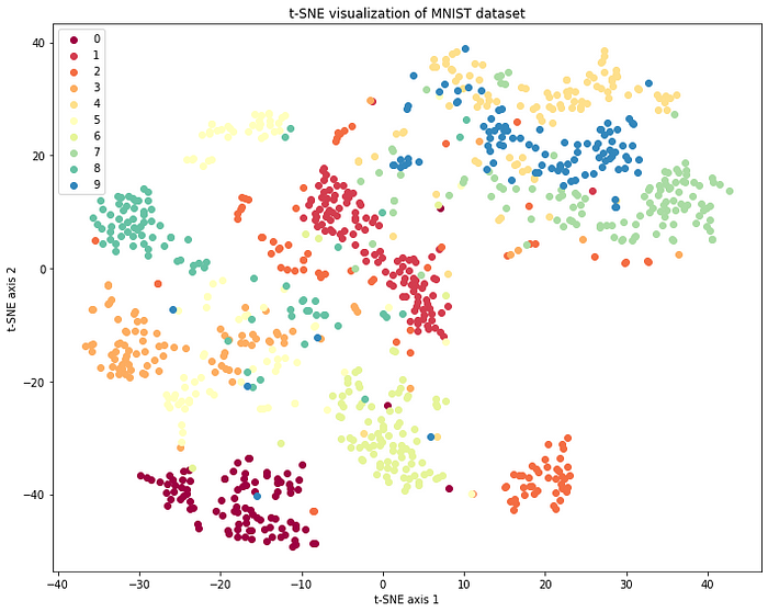

MNIST 2D Data Visualization using t-SNE

In this MNIST plot, we can observe clusters of similar digits. For example, the 0s are grouped together, and the 1s are grouped together, and so on. This indicates that the t-SNE algorithm has successfully captured the similarity structure in the high-dimensional MNIST data.

Note that the axes are centered around 0 because the t-SNE algorithm minimizes the distance between instances in the high-dimensional space and their projections in the 2D space, so that the resulting plot is optimized for visualizing the relationships between instances.

By visualizing the data in this way, it may be easier to identify patterns, groupings or similarities in the data that were not easily recognizable from the raw data. Additionally, it provides a way to explore and understand complex, high-dimensional datasets in a more intuitive way.

Applications of t-SNE

t-SNE is utilized extensively in numerous disciplines, including computer science, biology, neuroscience, and the social sciences. It is frequently employed to visualize high-dimensional data, such as images, videos, audio signals, and texts, and for exploratory data analysis and feature engineering.

1. Image recognition: t-SNE has been used to visualize the intermediate activations of Convolutional Neural Networks (CNNs) trained on image datasets, helping researchers understand how the networks learn and recognize patterns in images.
2. Natural language processing: t-SNE has been used to visualize the high-dimensional representations of words and documents, making it easier to understand the relationships between them and identify patterns in the data.
3. Genomics: t-SNE has been used to visualize high-dimensional gene expression data, enabling researchers to identify subtypes of diseases and understand the underlying biology.
4. Healthcare: t-SNE has been used to visualize electronic health records (EHRs), helping healthcare professionals identify patterns in patient data and make more informed decisions about diagnosis and treatment.
5. Marketing: t-SNE has been used to visualize customer data, enabling companies to segment their target audience and identify patterns in customer behavior.
6. Fraud detection: t-SNE has been used to visualize fraudulent transactions, making it easier to identify unusual patterns and detect fraudulent activity.

These are just a few common real-world scenarios where t-SNE has proved to be very beneficial, but the scope of using t-SNE extends far beyond.

Conclusion

In conclusion, t-SNE is an effective method for visualizing high-dimensional data that can assist uncover patterns, relationships, and clusters in complicated and multidimensional data. t-SNE’s ability to capture complicated, non-linear relationships between data points is one of its primary features, making it particularly helpful for visualizing high-dimensional data. In addition, it is highly efficient at discovering clusters in the data, even when the clusters are difficult to discern in the high-dimensional space.

If you find this article useful, please follow me for more such related content, where I frequently post about Data Science, Machine Learning and Artificial Intelligence.