Running Totals, and Moving Averages

During interviews, it has been observed that the interviewer can perplex candidates by asking them how to calculate running totals or moving averages. As a result, understanding and learning how to perform these complex computations becomes crucial. So, grab a cup of coffee and let’s go through these topics in such a way that you will never be perplexed about them in interviews.

Sliding Window

Introduction

Running Totals

So, what is a running total anyway you’d ask?

Glad you asked! Well a running total is just a fancy way of saying cumulative sum. A running total is a cumulative sum of a set of values that is calculated incrementally as new values are added to the set. It provides a running count of the sum of the values up to a certain point, allowing for an understanding of the trend or pattern in the data.

Where is running totals used?

Running totals is a very important key metric are useful for analyzing trends and patterns in data that accumulate over time. They can be used to gain insights into how a certain metric or feature is evolving over time. They are used by a wide range of professionals and industries, including:

1. Finance and Accounting: Running totals can be used to track the accumulation of expenses, revenue, or profits over a period of time.
2. Supply Chain Management: Running totals can be used to track the cumulative quantity of goods received, shipped, or in inventory over time.
3. Marketing and Sales: Running totals can be used to track the cumulative number of leads generated, sales made, or customer engagement over time.
4. Healthcare: Running totals can be used to track the accumulation of patient visits, medication doses, or treatment outcomes over time.
5. Sports: Running totals can be used to track the cumulative statistics for individual players, teams, or entire leagues over time.

It is very likely that you might be working in any of these domains, or your managers, stakeholders belong to or work with people from these departments and require this important metric to comprehend or report the flow of activities to higher management.

Moving Average

A moving average, also known as a running mean or cumulative mean, is a calculation of the mean of a dataset taken over a sliding window of a specified size. The sliding window is moved along the data points, so that at each step, the mean of the most recent data points within the window is calculated. This provides a smoothed representation of the data over time, which can help to remove fluctuations and highlight trends. The cumulative mean can be useful for financial and economic analysis, trend forecasting, and signal processing, among other applications.

Implementation

Okay, so you now have a good understanding of what these metrics are. Let’s not spend any more time and jump right into the coding to see how we can incorporate these strategies into our computations.

As usual, we will begin by building a dummy dataset containing Sales data for irregularly spaced timeseries of two weeks with missing data at random and then attempt to apply these strategies in Python using Pandas.

import pandas as pd
import numpy as np
import datetime as dt

# Create a sample dataframe with irregularly spaced time series data
dates = ['2023-01-01', '2023-01-03', '2023-01-05', '2023-01-07', '2023-01-07', '2023-01-08', '2023-01-09', '2023-01-10', '2023-01-12', '2023-01-15']
dates = [dt.datetime.strptime(x, '%Y-%m-%d') for x in dates]
df = pd.DataFrame({'Sales': [11, 22, np.nan, 14, 24, 25, 42, 34, np.nan, 14]}, index=dates)

This is how our original data looks like:

Raw Sales Data

Handling missing values in timeseries

As you can see, not only is there missing data in the recorded transactions in this dataset, but the timeseries is also irregular, i.e., there are dates for which the entire observation set is absent. For the interest of clarity, we will expand our timeseries to include all missing dates and attempt to interpolate the values for these missing data. If you are new to data imputation techniques, I recommend reading my earlier article on Data Imputation Techniques, in which I explored the majority of the commonly used as well as sophisticated techniques in data imputation. In this post, we’ll make certain assumptions about the underlying data and then utilize interpolation to fill in the missing information.

Resampling the data

# Resample the data to daily frequency
df = df.resample('D').mean()

Now our dataset looks like:

Resampled Data

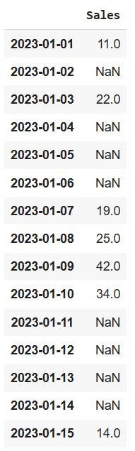
We have now successfully resampled the irregular timeseries to a regular timeseries of daily frequency. But now we have more missing values than we started with. We will proceed with filling these missing values with interpolation, however, this is not a recommended method, as it induces bias in the data.

Caveats

The best method for computing cumulative aggregations for irregularly spaced time series data depends on the specifics of your data and what you are trying to achieve.

Interpolating NaN values and then computing aggregations is a common approach when working with irregularly spaced time series data. Interpolation allows you to fill in missing values based on the values of surrounding data points, which can give you a more complete and accurate representation of the underlying trends in your data. The cumulative mean can then be calculated as the running average of all data points.

However, there are some potential downsides to this approach. Interpolation can introduce bias into your data, as it relies on assumptions about the behavior of the underlying trends in your data. Additionally, if there are large gaps in your data or if the underlying trends are complex, interpolation may not accurately fill in the missing values.

On the other hand, leaving NaN values as is may be a better approach if your data is sparse or if there is little information about the underlying trends in your data. This approach can be less prone to bias, as it does not make any assumptions about the data. However, if you have a large number of NaN values or if the underlying trends in your data are important, this approach may not provide a complete or accurate representation of your data.

Ultimately, the choice of method will depend on the specifics of your data, the goals of your analysis, and the assumptions you are willing to make about the underlying trends in your data.

Interpolation

# Interpolate missing values
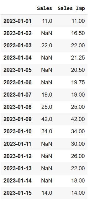
df['Sales_Imp'] = df['Sales'].interpolate(method='linear')

Now, our dataset looks like below, where we have added another column which contains the imputed values as ‘Sales_Imp’:

Imputed Data

Rolling Totals

# Calculate cumulative sum
df['Cum_sum_orig'] = df['Sales'].cumsum().where(df['Sales'].notna(), np.nan)
df['Cum_sum_imp'] = df['Sales_Imp'].cumsum()

Rolling Totals Calculated

We can see that imputing the values smoothed our data points, but if you look at the final cumulative sum on ‘2023–01–15,’ you will see that our sum grew by more than double for the imputed data. This is a critical decision that must be made before imputing the missing values, as it can frequently inject bias into the data.

Moving Average

# Calculate cumulative mean
df['Cum_mean_orig'] = df['Sales'].expanding().mean().where(df['Sales'].notna(), np.nan)
df['Cum_mean_imp'] = df['Sales_Imp'].expanding().mean()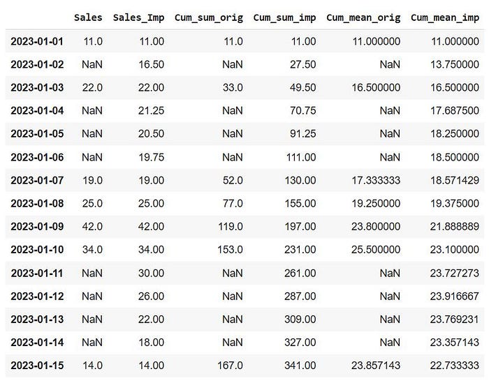

Moving Averages

We can now clearly determine what happened to our data. This is the outcome of interpolation. We can easily observe that the imputation has had a significant impact on the moving average. If we hadn’t used interpolation to impute the data, our moving averages would be markedly different and a more accurate representation of the actual data. As mentioned above, this choice completely depends on the context of the problem. If there are large number of missing data with patterns which are difficult to interpret (as the case with this example) a common choice would be to interpolate, keeping in mind that it might not be an accurate representation of the actual data, but it would definitely provide a more “smoothed” representation of the patterns and trends in the data.

Moving Average using Sliding Window

Another common technique of computing moving averages involves taking a rolling average of a certain number of observations. In pandas, the rolling function can be used to create a rolling window, and various aggregation functions can be applied to the window. For example, the following code calculates a rolling mean with a window size of 3:

# Calculate Moving Average using Rolling Mean
df['Rolling_Mean_imp'] = df['Sales_Imp'].rolling(window=3).mean()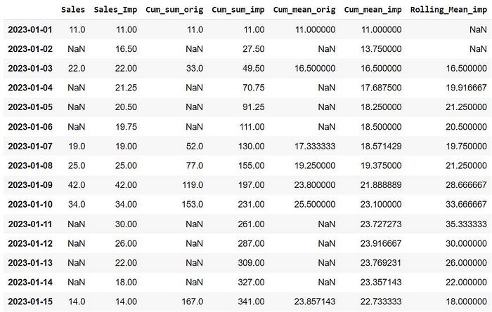

Rolling Mean

Now, we have calculated the moving average by slicing the data points into “window” of 3 observations at a time and calculating the mean of this window. Then this window is shifted by one record at a time downwards and the mean in calculated on the new window. The choice of window size depends completely on the context of the problem. For example, for weekly patterns, one might opt for a window size of 7. Also, note the first 2 observations have a rolling mean of NaN, as the data required for calculating these values are the previous two days (which is not present) because they are the first two records of the dataset. In general, using rolling mean of window size ‘m’ will always contain atleast ‘m-1’ missing data.

Considerations

Computing cumulative mean in pandas can be achieved in several ways, depending on the type of data you are working with and the desired output. Here are some of the details to consider when computing cumulative mean in pandas:

1. Data type: It’s important to know whether you are working with time-series data, categorical data, or numerical data as this will affect the type of aggregation you should perform. For example, with time-series data, it’s common to compute a running or cumulative mean by resampling the data and computing the mean of each resampled period.
2. Missing values: Missing values can affect the computation of cumulative mean in pandas. It is important to decide whether to interpolate missing values before computing the cumulative mean or to leave them as is. Interpolation of missing values can lead to biased results if the missing values are not representative of the underlying data distribution. On the other hand, leaving missing values as is may result in a cumulative mean that does not capture the true underlying distribution.
3. Frequency: When computing cumulative mean for time-series data, it’s important to determine the frequency at which to compute the mean. The frequency can be daily, weekly, monthly, or any other frequency that makes sense for your data. When resampling the data, the cumulative mean can be computed as the mean of each resampled period.
4. Window size: The window size is the number of consecutive values used to compute the cumulative mean. The window size can be adjusted to achieve the desired level of smoothing or aggregation. When using a sliding window approach, it’s important to specify the window size and the step size (the number of steps between consecutive windows).
5. Aggregation method: The type of aggregation to perform when computing cumulative mean in pandas can vary depending on the data type and desired output. For example, when working with numerical data, the mean can be computed as the average of the values in the window. For categorical data, the mode (the most frequent value) or the count of each category can be used.

Conclusion

In conclusion, computing cumulative mean in pandas can be a complex operation that requires careful consideration of the data type, missing values, frequency, window size, and aggregation method. It’s important to understand the trade-offs and limitations of each approach to ensure accurate results.

You should now have a solid knowledge of how rolling totals and moving averages are computed, as well as the different decisions that must be made in order to accomplish these complex computations. It is critical that these judgments are made in the context of the problem, and that a discussion with stakeholders is held if necessary to determine the granularity of the expected outcome. Any modification in these variables could cause major variations in the observed outcome. It is recommended that you revisit the considerations section above before actually implementing these methods.

If you find this article useful, please follow me for more such related content, where I frequently post about Data Science, Machine Learning and Artificial Intelligence.