Gradient Descent and Regression

The most frequently asked question in Data Science interviews is about gradient descent. Finding the gradient of a function is maybe the most crucial idea in all of machine learning. Because gradient descent is critical, we will attempt to comprehend it mathematically in depth in this article. Since there are abundant resources available online for the coding syntax, I shall not be providing the codes in this article, instead we will focus only on the math. A word of caution: this article contains a lot of math, so avid readers are requested to look up commonly used math notations online.

Gradient Descent Algorithm [1]

Gradient

The gradient of a scalar function f(x) is a vector that points in the direction of the maximum rate of increase of the function. In other words, it is the vector of partial derivatives of the function with respect to its variables. The gradient of f(x) is denoted as ∇f(x) and is defined as:

Gradient of a function

where x = [x1, x2, …, xn]^T and n is the number of variables.

Properties of Gradients

Some properties of gradient include:

Additive property: The additive property of gradients states that the gradient of a sum of functions is equal to the sum of the gradients of the individual functions.

Additive Property of Gradients

Scalar Multiplication: The scalar multiplication property of gradients states that the gradient of a scalar-multiplied function is equal to the scalar times the gradient of the original function.

Scalar Multiplication Property of Gradients

Associative Property: The associative property of gradients states that the gradient of a composed function is equal to the gradient of the inner function evaluated at the output of the outer function, multiplied by the gradient of the outer function evaluated at the same output.

Associative Property of Gradients

Gradient of Euclidean Norm: The gradient of the squared Euclidean norm of a vector x with respect to x is equal to 2x, which is a scalar multiple of the original vector. This result is important in optimization and machine learning, where the squared Euclidean norm is often used as a loss or cost function.

Gradient of Euclidean Norm

Gradient of Quadratic Form: The gradient of the quadratic form x^T A x with respect to x is equal to (A + A^T) x, where A is a symmetric matrix.

Gradient of Quadratic Form

Gradient of Hadamard Product: The Hadamard product, also known as the element-wise product, of two functions is defined as the point-wise product of the values of the functions at a given point. If f(x) and g(x) are two functions, their Hadamard product is denoted as h(x) = f(x) * g(x). The gradient of the Hadamard product of two functions can be calculated using the chain rule of differentiation, and the result is the element-wise sum of the product of each function and its gradient.

Gradient of Hadamard Product

Leibniz’s rule: Leibniz’s rule states that the derivative of an implicit function with respect to its inputs is given by the inverse of its Jacobian matrix, which relates the change in the output of the function to the change in its inputs.

Leibniz’s rule

Regression

Regression is a statistical method used to model the relationship between a dependent variable and one or more independent variables. It is used to make predictions about the dependent variable based on the values of the independent variables.

Let X be a matrix of independent variables and Y be a vector of dependent variables. The goal of regression is to find a linear relationship between X and Y, represented by a vector of coefficients θ.

Hypothesis Function

In this equation, h_θ(x_i) represents the hypothesis function for the i-th instance, given the feature vector x_i and the coefficients θ. The hat symbol (^) is used to indicate an estimated or predicted value.

The equation h_θ(x_i) = θ^T x_i shows that the predicted value is obtained by taking the dot product of the feature vector x_i and the coefficients θ. This results in a scalar value, which represents the predicted value for the dependent variable. The errors from the predictions are measured using the loss function L = y_i — y^.

In linear regression, the goal is to find the coefficients θ that minimize the difference between the predicted values and the actual values, as measured by some cost function J(θ), such as the mean squared error.

Cost Function

It order to find the optimal value of the coefficient vector θ*, we need to find the index of the loss function

Optimal Coefficient

The estimated coefficients can then be used to make predictions on new data.

The L2 norm is a common choice of cost function where

Optimal Theta using L2 Norm Cost Function

The same equation can also represented in closed form or Normal form as:

L2 Norm Cost Function in Closed form

The optimal value of coefficient can also be shown to be:

Optimal Coefficient in closed form

Caveats:

1. Computing the inverse of a matrix has a cubic time complexity.
2. (X^T.X) should be full rank to be invertible.

Matrix Inversion Problem

Gradient Descent

Finally, now we are in a good position to understand the gradient descent algorithm mathematically.

Gradient descent is an optimization algorithm used to find the minimum of a cost function. It is widely used in machine learning to estimate the parameters of a model, such as the coefficients in linear regression or the weights in neural networks.

The idea behind gradient descent is to iteratively update the parameters in the direction of the negative gradient of the cost function, in order to reduce its value and find the minimum. The gradient of the cost function with respect to the parameters represents the direction of steepest ascent, so moving in the opposite direction, i.e., the negative gradient, will lead towards the minimum.

Mathematically, gradient descent can be written as:

Gradient Descent Algorithm

where:

• θ_j is the j-th parameter in the vector of parameters θ
• J(θ) is the cost function
• ∇_θ J(θ) is the gradient of the cost function with respect to the parameters θ
• α is the learning rate, a scalar that determines the step size for each iteration
• m is the number of training examples

The gradient of the cost function with respect to the parameters can be calculated using the chain rule of differentiation. For example, in linear regression, the cost function is the mean squared error:

Linear Regression Cost Function

The gradient of this cost function can be found to be:

Gradient for linear regression

Steps in Gradient Descent

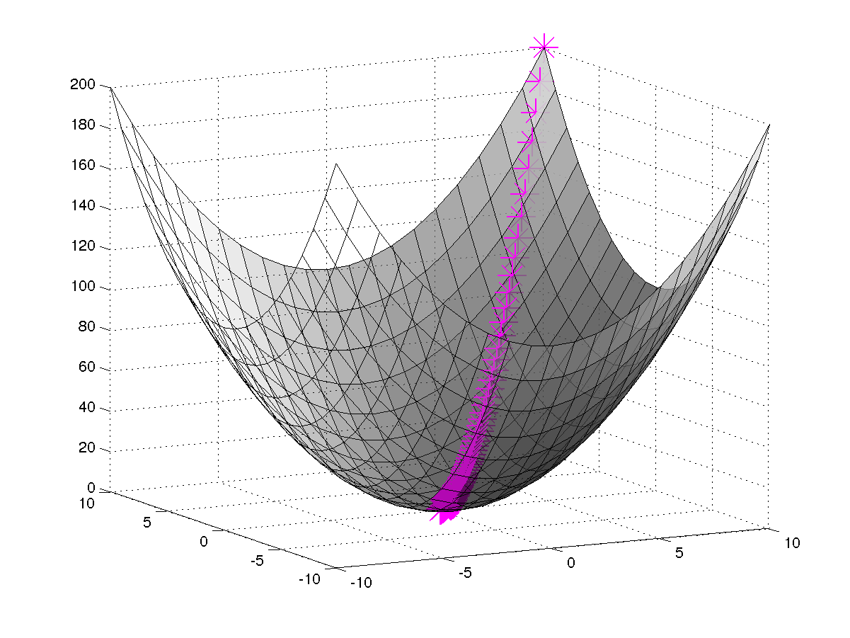
The gradient descent algorithm starts with an initial guess for the parameters, and then repeatedly updates the parameters in the direction of the negative gradient until convergence. The convergence criteria is typically based on the change in the cost function value from one iteration to the next. Let us see the steps using Normal form equation

Gradient Descent Steps

The convergence can be met if any of the following is satisfied:

1. gradient becomes zero
2. the algorithm has reached the maximum number of iterations
3. the change in coefficients is very minor in consecutive iterations (~0.00001)
4. the change in cost function is very minor in consecutive iterations (~0.00001)

Disadvantages of Gradient Descent

Gradient descent is a simple and effective optimization algorithm for many problems, but it also has some drawbacks and limitations. Some of the main cons of gradient descent are:

1. Convergence rate: Gradient descent can be slow to converge, especially for complex and high-dimensional cost functions. The convergence rate can also be affected by the choice of the learning rate and the presence of local minima.
2. Local minima: Gradient descent is sensitive to the presence of local minima in the cost function, which can lead to getting stuck in a suboptimal solution. To mitigate this issue, different variations of gradient descent, such as stochastic gradient descent, mini-batch gradient descent, and momentum optimization, have been developed.
3. Hyperparameters: Gradient descent requires setting the learning rate, which can be difficult to tune. If the learning rate is too high, the algorithm may oscillate and not converge, while if the learning rate is too low, the convergence rate can be very slow.
4. Requires scaling: Gradient descent assumes that the features are on a similar scale, so it is necessary to normalize the input data before applying the algorithm. If the data is not properly scaled, the convergence rate can be slow or the algorithm may not converge at all.
5. Sensitive to initialization: The initial guess for the parameters can have a large impact on the convergence of the algorithm, especially if the cost function is non-convex. To mitigate this issue, different initialization techniques, such as random initialization or pre-training, can be used.
6. Computationally Expensive: Gradient descent is a batch optimization algorithm, which means that it requires a large amount of data to estimate the gradient. This can be computationally expensive and memory-intensive, especially for high-dimensional problems.
7. Not suitable for non-differentiable functions: Gradient descent relies on computing the gradient of the cost function, which requires it to be differentiable. If the cost function is not differentiable, gradient descent cannot be used directly.
8. Sensitive to the choice of the cost function: The performance of gradient descent can be greatly influenced by the choice of the cost function, and it may not work well for all types of problems. For example, gradient descent may struggle to optimize cost functions that are highly non-linear or have many local minima.

Conclusion

In conclusion, gradient descent is a widely used optimization algorithm that has its limitations and can be challenging to use in some cases. However, it is still a powerful tool for and widely used optimization algorithm in many applications, including machine learning, deep learning, optimization, and it continues to be an active area of research and development.

Congratulations on making it this far. You should now have a solid mathematical knowledge of the gradient descent algorithm and regression in general. You should be able to explain the algorithm’s steps using both calculus and linear algebra by now. Because of the numerous drawbacks of gradient descent, researchers prefer to employ more complex gradient descent methods such as stochastic gradient descent, robust regression, ridge and lasso regression, and many others, but that is a topic for the next article.

If you find this article useful, please follow me for more such related content, where I frequently post about Data Science, Machine Learning and Artificial Intelligence.

Reference:

1. simar (2023). Gradient Descent Visualization (https://www.mathworks.com/matlabcentral/fileexchange/35389-gradient-descent-visualization), MATLAB Central File Exchange. Retrieved January 30, 2023.